Detailed Description

Tutorials for ebsd.

Tutorials

Example: Read EBSD data and plot the ND IPF

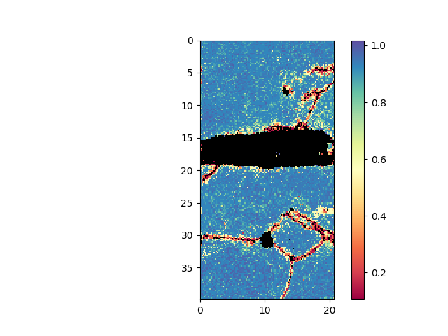
plot confidence index (CI). Mask out all points with a CI less than 0.1. Initially all points are present in the mask, i.e. they are shown. By masking out points, these are removed from the mask.
plot inverse pole figure in normal direction
play with different options (1024pixel to see speed of plotting)
setVMask: for fast plotting;
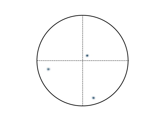
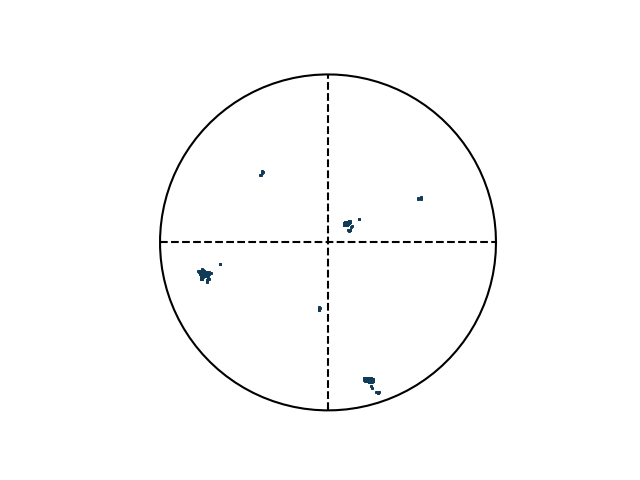
pole figure (PF) in the [1,0,0] direction. The OIM software has the top left corner has coordinate origin

>>> from ebsd import EBSD
>>> e = EBSD("Examples/EBSD.ang")
Load .ang file:  Examples/EBSD.ang
   Read file with step size: 0.2 0.2
   Optimal image pixel size: 103
   Number of points: 23909
>>> e.plot(e.CI)

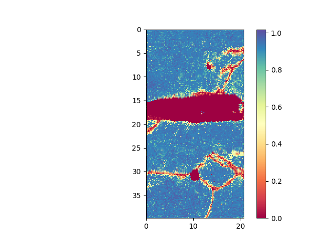
>>> e.maskCI( 0.1 )
>>> e.plot( e.CI )

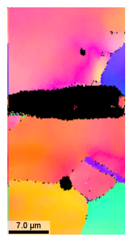
>>> e.plotIPF()

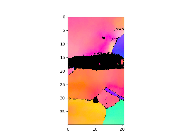
>>> e.plotIPF(1024)

>>> e.addScaleBar()

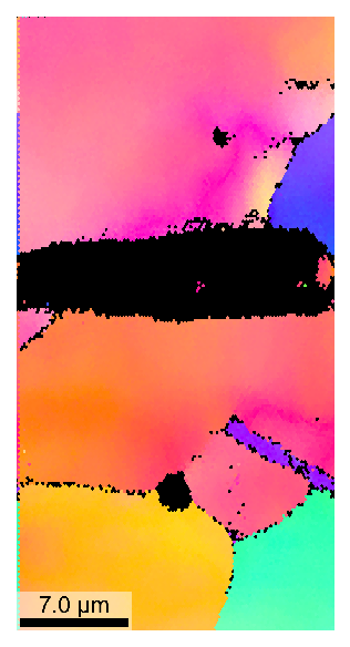
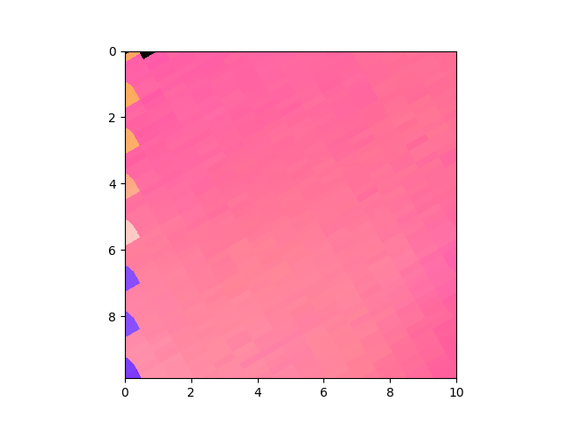
>>> e.setVMask(4)                          # use only every 4th point, increases plotting speed
>>> e.plotIPF(1024)

>>> e.cropVMask(0,0,10,10)               # show only a section of the image, increases plotting speed
>>> e.plotIPF(1024)

>>> e.plotPF([1,0,0])

>>> e.plotPF([1,0,0],points=True)

Example: Interaction with OIM Software to update grain information from different file

How to export txt-file from OIM that can be read:

Partition->export-> grain file -> use "grain file type 1" (saves a txt file)
Partition->export-> partition data -> save as .ang

Warning: This is example input file does not exist, anymore. Not tested

> e = EBSD("Examples/Test.ang")
> e.loadTXT("Examples/TestB.txt")
> e.maskCI(0.1)
> e.removePointsOfMask()
> e.writeANG("ebsd.ang")

Which can then be read in OIM again

Compare with OIM software and verify pole-figure

>>> import numpy as np
>>> from ebsd import EBSD
>>> from ebsd_Orientation import Orientation
>>> e = EBSD("Examples/EBSD.ang")
Load .ang file:  Examples/EBSD.ang
   Read file with step size: 0.2 0.2
   Optimal image pixel size: 103
   Number of points: 23909
>>> e.maskCI( 0.001 )
>>> e.plotIPF('ND')                        
>>> e.cropVMask(xmin=18,ymin=12,ymax=17)
>>> e.plotIPF('ND')

Inspect the original data at x,y = 20.1,14.38 um
line 8785 from EBSD.ang
5.55763 2.18448 3.83349 20.10000 14.37602 3653.496 0.482 0 1 1.104

>>> print (np.degrees([ 5.55763, 2.18448, 3.83349]))
[318.4287431  125.16148443 219.64279781]
>>> e.cropVMask(xmin=20,xmax=20.2,ymin=14.3,ymax=14.4)
>>> e.y[e.vMask]                           #verify y: correct if rounding accounted for
array([14.37602])
>>> angle = e.quaternions[e.vMask].asEulers().flatten()
>>> print (np.round(np.degrees(angle)))                #convert to only positive values
[ -42.  125. -140.]
>>> print (np.round(np.degrees(angle)+np.array([360,0,360])))
[318. 125. 220.]

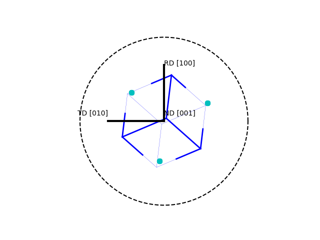
Plot correct unit cells and pole-figures using the orientation-class

>>> o = Orientation(Eulers=angle, symmetry="cubic")
>>> o.toScreen()                                   #first item is one looking for 
>>> o.plot(plot2D='up-left')

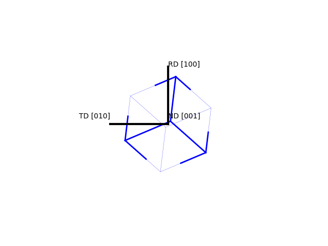
>>> o.plot(poles=[1,0,0],plot2D='up-left',scale=1.5)

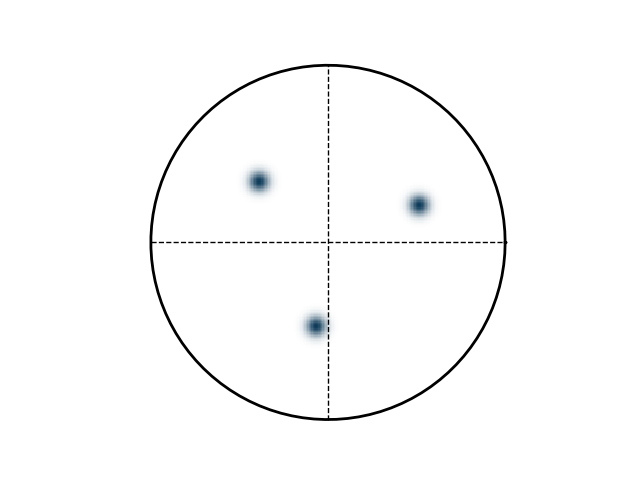
Create artificial ebsd pattern to check PF

>>> e = EBSD('void318.|125.|219.6|0|2')
Void mode 318.|125.|219.6|0|2
   Euler angles: 5.55 2.18 3.83 | distribution: 0.0 | numberPerAxis: 2.0
   Read file with step size: 1.0 1.0
   Optimal image pixel size: 1
   Number of points: 4
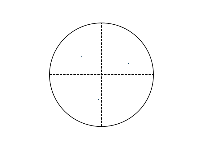
>>> e.plotPF(size=5)

>>> e.plotPF(points=True)

Finally, inspect pole-figure of data and compare OIM software, mTex and this python code

>>> e = EBSD("Examples/EBSD.ang")
Load .ang file:  Examples/EBSD.ang
   Read file with step size: 0.2 0.2
   Optimal image pixel size: 103
   Number of points: 23909
>>> e.maskCI( 0.001 )
>>> e.plotPF(size=1)                       
>>> e.plotPF()                 
>>> e.plotPF(proj2D='down-right')

description	OIM software	mTex software	this python code
IPF ND*
IPF RD		I cannot produce
PF [100]
PF [100] contour	I cannot produce
PF [111]

Issues from mTex:

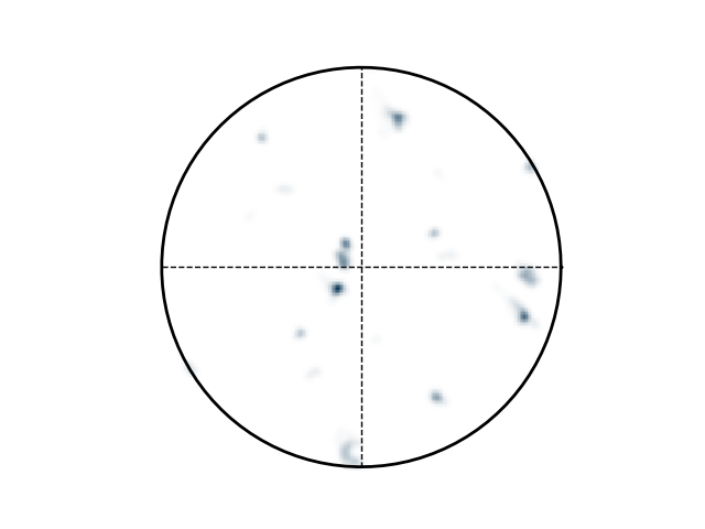
.bmp (left): low color number when exporting from external window. .png works (right)
Explicitly select x-axis as North and z-axis as outOfPlane; normal orientation has different result, although it should be the same

Average orientation in file, does not make sence for this multi-grain case

averaging takes lots of time: Orientation.average()

>>> from ebsd_Orientation import Orientation
>>> from ebsd import EBSD
>>> Orients = []
>>> e = EBSD("Examples/EBSD.ang")
Load .ang file:  Examples/EBSD.ang
   Read file with step size: 0.2 0.2
   Optimal image pixel size: 103
   Number of points: 23909
>>> for i in range(len(e.x)):
...   Orients.append(Orientation(quaternion=e.quaternions[i], symmetry="cubic"))
>>> avg = Orientation.average( Orients)
>>> print ("Average orientation",np.round(avg.asEulers(degrees=True, standardRange=True),0))

Compare the three software for bicrystal

description	OIM software	mTex software	this python code
IPF ND*
IPF RD		I cannot produce
PF [100]

Python code

>>> from ebsd import EBSD
>>> e = EBSD("Examples/EBSD.ang")
Load .ang file:  Examples/EBSD.ang
   Read file with step size: 0.2 0.2
   Optimal image pixel size: 103
   Number of points: 23909
>>> e.cropVMask(ymin=35)
>>> e.addSymbol(5,37, scale=2)

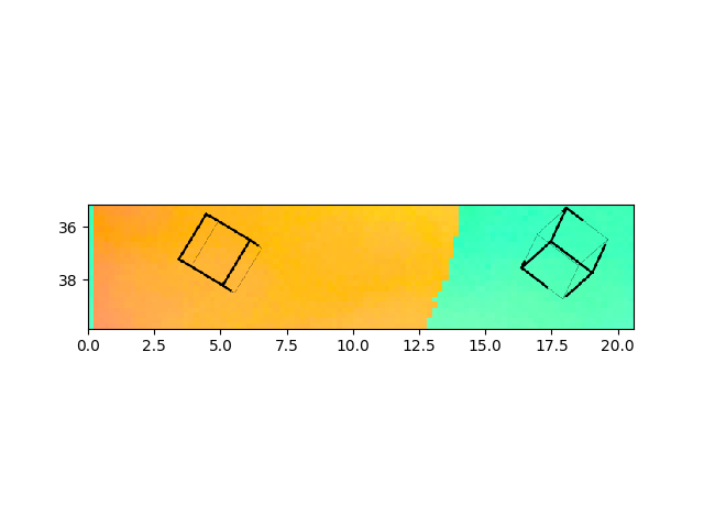
>>> e.plotIPF("RD",fileName="pythonRD.png")
>>> e.addSymbol(5,37, scale=2)
>>> e.addSymbol(18,37, scale=2,fileName="pythonRD.png")

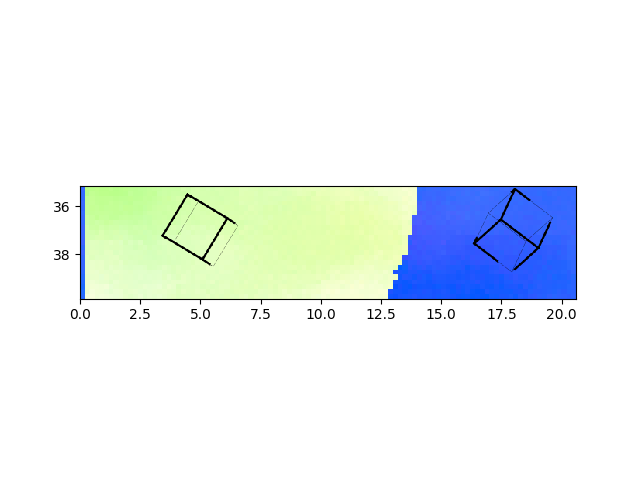
>>> e.plotIPF("TD",fileName="pythonTD.png")
>>> e.addSymbol(5,37, scale=2)
>>> e.addSymbol(18,37, scale=2,fileName="pythonTD.png")

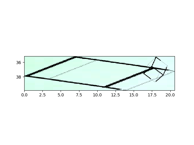
>>> e.plotPF(      fileName="pythonPF.png")

please, note, the last image is not colored. This is not implemented yet. TODO

how to run mTex

>> startup_mtex
>> import_wizard('ebsd')
% and select EBSD.osc
% select plotting convention 5: x-to-right; y-to-bottom
% select "convert Euler 2 Spacial Referecence Frame"
% save to workspace variable
>> csCopper = ebsd('Cu').CS;
>> plot(ebsd('Cu'),ebsd('Cu').orientations,'coordinates','on')
>> cS = crystalShape.cube(ebsd.CS)
>> region = [0 35 50 50];
>> ebsdC  = ebsd(inpolygon(ebsd,region))
>> plot(ebsdC('Cu'),ebsdC('Cu').orientations,'coordinates','on')
>> plotPDF(ebsd('Cu').orientations, Miller({1 0 0},csCopper))
% select xNorth zOutOfPlane as axis in mTex
>> plotPDF(ebsd('Cu').orientations, Miller({1 1 1},csCopper))
>> odf = calcODF(ebsd('Cu').orientations)
>> plotPDF(odf,Miller({1 0 0},csCopper) )

If separate window: save as png, because bmp colorscale is broken

if not separet window: save as bmp, because png crops sections off select xNorth zOutOfPlane as axis in mTex
compare to original which should be the same

Data that exists and can be used for plotting in plot:

OIM software:
- e.phi1, e.PHI, e.phi2 : Euler angles saved as quaternions
- e.x, e.y : x,y coordinates
- e.IQ, e.CI, e.phaseID : Image Quality, confidence index (bad=0 ... good=1) , phase id
- e.SEMsignal : SEM signal
- e.fit :
Oxford:
- bc: band contrast

Hints for developers

run ./verifyAll.py after all changes to verify the code and create the html-documentation
git commands
- git add -A
- git gui
- git commit -m "solved symbolic link issue"
- git push -u origin master